布林通道交易策略

Mar 21 2023

本文重点概要

文章难度：★☆☆☆☆

以均线（ MA ）以及其正负标准差组成布林通道的上界、下界，透过这三条线绘制出布林通道，判断进场、出场时机。

前言

布林通道（Bollinger Band）是由 John Bollinger 在1980 年代所发明的技术指标。布林通道是由均线和统计学的标准差概念结合而成，均线 (Moving Average)，简称 MA，代表过去一段时间的平均成交价格，一般来说在布林中使用的时间区段为近20日；标准差 (Standard Deviation)，简称SD，常以σ作为代号，用于表示资料中数值的分散程度。

布林通道总共包含三条线：
● 上轨：20 MA＋2 倍标准差
● 中轨：20 MA
● 下轨：20 MA — 2 倍标准差

由于在长时间观测下，标的价格的变化会呈现常态分布 (Normal Distribution)，而根据统计学原理，在常态分布下有95%的机率，资料会分布在平均值正负两倍标准差(μ − 2σ, μ + 2σ)之间，也称为95%的信赖区间，而布林通道正是以上述的统计学原理作为理论依据，发展出来的技术指标。

实际策略如下：

当收盘价触碰到上界时，视为接下来可能会下跌的讯号，以隔日开盘价抛售持有部位。

当收盘价触碰到下界时，视为接下来有可能谷底反弹的讯号，以隔日开盘价买入一单位。当满足上述条件时，以及满足本金充足、已持有部位与当日收盘价低于上次买入讯号收盘价时，则继续加码一单位。

编辑环境及模组需求

本文使用Mac OS并以jupyter作为编辑器

import pandas as pd 
import re
import numpy as np 
import tejapi
from functools import reduce
import matplotlib.pyplot as plt
from collections import defaultdict, OrderedDict
from tqdm import trange, tqdm
import plotly.express as px
import plotly.graph_objects as go

tejapi.ApiConfig.api_key = "Your Key"
tejapi.ApiConfig.ignoretz = True

资料库使用

上市(柜)调整股价(日)-均价、未调整(日)技术指标

资料导入

资料期间从2021–06–01至2022–12–31，以友达光电(2409)作为实例，抓取未调整的收盘价、BB-Upper(20)、BB-Lower(20)资料，并以报酬指数(Y9997)作为大盘进行绩效比较。

stock = tejapi.get('TWN/APRCD',
                   paginate = True,
                   coid = '2409',
                   mdate = {'gte':'2021-06-01', 'lte':'2022-12-31'},
                   opts = {
                       'columns':[ 'mdate', 'open_d', 'high_d', 'low_d', 'close_d', 'volume']
                   }
                  )

ta = tejapi.get('TWN/AVIEW1',
                paginate = True,
                coid = '2409',
                mdate = {'gte':'2021-06-01', 'lte':'2022-12-31'},
                opts = {
                    'columns':[  'mdate', 'bbu20', 'bbma20', 'bbl20']
                }
               )

market = tejapi.get('TWN/APRCD',
                   paginate = True,
                   coid = "Y9997",
                   mdate = {'gte':'2021-06-01', 'lte':'2022-12-31'},
                   opts = {
                       'columns':[ 'mdate', 'close_d', 'volume']
                   }
                  )

#将标的价格资讯与技术指标资讯以日期进行合并
data = stock.merge(ta, on = ['mdate'])
#将大盘价格资讯进行重新命名，与标的资料区别
market.columns = ['mdate', 'close_m', 'volume_m']
#将日期设为指标
data = data.set_index('mdate')

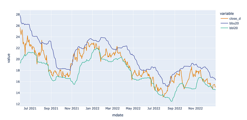
取得股价与技术指标资料后我们首先来绘制布林通道，这里使用plotly.express来进行图表的绘制。其中bbu20为20日布林通道上界、bbl20为通道的下界，而close_d为收盘价。

fig = px.line(data,   
            x=data.index, 
            y=["close_d","bbu20","bbl20"], 
            color_discrete_sequence = px.colors.qualitative.Vivid
            )
fig.show()

交易策略

这里我们定义了几个参数
● principal：本金
● position：股票部位持有张数
● cash：现金部位持有量
● order_unit：交易单位数

principal = 500000
cash = principal
position = 0
order_unit = 0
trade_book = pd.DataFrame()

for i in range(data.shape[0] -2):
    
    cu_time = data.index[i]
    cu_close = data.loc[cu_time, 'close_d']
    cu_bbl, cu_bbu = data.loc[cu_time, 'bbl20'], data.loc[cu_time, 'bbu20']
    n_time = data.index[i + 1]
    n_open = data['open_d'][i + 1]
    
    
    if position == 0: #进场条件
        if cu_close <= cu_bbl and cash >= n_open*1000: 
            position += 1
            order_time = n_time
            order_price = n_open
            order_unit = 1
            friction_cost = (20 if order_price*1000*0.001425 < 20 else order_price*1000*0.001425)
            total_cost = -1 * order_price * 1000 - friction_cost
            cash += total_cost
            trade_book = trade_book.append(
                pd.Series(
                [
                    stock_id, 'Buy', order_time, 0, total_cost, order_unit, position, cash
                ]), ignore_index = True)
            
    elif position > 0:
        if cu_close >= cu_bbu: # 出场条件
            order_unit = position
            position = 0
            cover_time = n_time
            cover_price = n_open
            friction_cost = (20 if cover_price*order_unit*1000*0.001425 < 20 else cover_price*order_unit*1000*0.001425) + cover_price*order_unit*1000*0.003
            total_cost = cover_price*order_unit*1000-friction_cost
            cash += total_cost
            trade_book = trade_book.append(pd.Series([
                stock_id, 'Sell', 0, cover_time, total_cost, -1*order_unit, position, cash
            ]), ignore_index=True)
            
        elif cu_close <= cu_bbl and cu_close <= order_price and cash >= n_open*1000: #加码条件: 碰到下界，比过去买入价格贵
            order_unit = 1
            order_time = n_time
            order_price = n_open
            position += 1
            friction_cost = (20 if order_price*1000*0.001425 < 20 else order_price*1000*0.001425) 
            total_cost = -1 * order_price * 1000 - friction_cost
            cash += total_cost
            trade_book = trade_book.append(
            pd.Series(
            [
                stock_id, 'Buy', order_time, 0, total_cost, order_unit, position, cash
            ]), ignore_index = True)
            
if position > 0: # 最后一天平仓
    order_unit = position
    position = 0
    cover_price = data['open_d'][-1]
    cover_time = data.index[-1]
    friction_cost = (20 if cover_price*order_unit*1000*0.001425 < 20 else cover_price*order_unit*1000*0.001425) + cover_price*order_unit*1000*0.003
    cash += cover_price*order_unit*1000-friction_cost
    trade_book = trade_book.append(
    pd.Series(
    [
        stock_id, 'Sell',0, cover_time, cover_price*order_unit*1000-friction_cost, -1*order_unit, position, cash
    ]), ignore_index = True)    
    
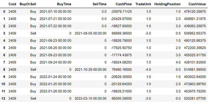
trade_book.columns = ['Coid', 'BuyOrSell', 'BuyTime', 'SellTime', 'CashFlow','TradeUnit', 'HoldingPosition', 'CashValue']

交易纪录

执行完上述的交易策略，接著就来看看在这段时间内我们进行交易资讯表，制作交易资讯表方法请详见程式码。
● BuyTime: 买入时间点
● SellTime: 卖出时间点
● CashFlow: 现金流出入量
● TradeUnit: 买进卖出张数
● HoldingPosition: 持有部位
● CashValue: 剩余现金量

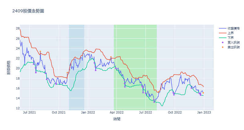
观察以下图表(绘图方法请见下方程式码)，可以发现在2021年11月到2021年12月的上升区段(图中浅蓝色区域)，由于收盘价无法碰触到布林通道下界，因此一直没有买入持有，导致无法赚取这区段的价差。

同样的问题也出现在连续下降波段，比如2022年4月开始的下降趋势(图中浅绿色区域)，不断地碰触布林通道下界，在回涨一小段后，因布林通道上界过低容易碰触到，所以很快就卖出掉，导致这段期间的交易为负报酬。

事实上，由于20日布林通道的迟滞性，故无法反映短期高波动的价格变化，若您所分析的股票为涨跌幅度较大者，建议缩短布林通道的期间或搭配其他观察趋势的指标建立交易策略。

绩效计算

cash = principal
data_ = data.copy()
data_ = data_.merge(trade_book_, on = 'mdate', how = 'outer').set_index('mdate')
data_ = data_.merge(market, on = 'mdate', how = 'inner').set_index('mdate')

# fillna after merge
data_['CashValue'].fillna(method = 'ffill', inplace=True)
data_['CashValue'].fillna(cash, inplace = True)
data_['TradeUnit'].fillna(0, inplace = True)
data_['HoldingPosition'] = data_['TradeUnit'].cumsum()

# Calc strategy value and return
data_["StockValue"] = [data_['open_d'][i] * data_['HoldingPosition'][i] *1000 for i in range(len(data_.index))]
data_['TotalValue'] = data_['CashValue'] + data_['StockValue']
data_['DailyValueChange'] = np.log(data_['TotalValue']) - np.log(data_['TotalValue']).shift(1)
data_['AccDailyReturn'] =  (data_['TotalValue']/cash - 1) *100

# Calc BuyHold return
data_['AccBHReturn'] = (data_['open_d']/data_['open_d'][0] -1) * 100

# Calc market return
data_['AccMarketReturn'] = (data_['close_m'] / data_['close_m'][0] - 1) *100

# Calc numerical output
overallreturn = round((data_['TotalValue'][-1] / cash - 1) *100, 4) # 总绩效
num_buy, num_sell = len([i for i in data_.BuyOrSell if i == "Buy"]), len([i for i in data_.BuyOrSell if i == "Sell"]) # 买入次数与卖出次数
num_trade = num_buy #交易次数

avg_hold_period, avg_return = [], []
tmp_period, tmp_return = [], []
for i in range(len(trade_book_['mdate'])):
    if trade_book_['BuyOrSell'][i] == 'Buy':
        tmp_period.append(trade_book_["mdate"][i])
        tmp_return.append(trade_book_['CashFlow'][i])
    else:
        sell_date = trade_book_["mdate"][i]
        sell_price = trade_book_['CashFlow'][i] / len(tmp_return)
        avg_hold_period += [sell_date - j for j in tmp_period]
        avg_return += [ abs(sell_price/j) -1  for j in tmp_return]
        tmp_period, tmp_return = [], []

avg_hold_period_, avg_return_ = np.mean(avg_hold_period), round(np.mean(avg_return) * 100,4) #平均持有期间，平均报酬
max_win, max_loss = round(max(avg_return)*100, 4) , round(min(avg_return)*100, 4) # 最大获利报酬，最大损失报酬
winning_rate = round(len([i for i in avg_return if i > 0]) / len(avg_return) *100, 4)#胜率
min_cash = round(min(data_['CashValue']),4) #最小现金持有量

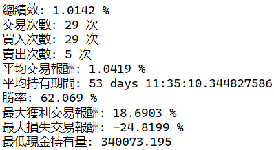
print('总绩效:', overallreturn, '%')
print('交易次数:', num_trade, '次')
print('买入次数:', num_buy, '次')
print('卖出次数:', num_sell, '次')
print('平均交易报酬:', avg_return_, '%')
print('平均持有期间:', avg_hold_period_ )
print('胜率:', winning_rate, '%' )
print('最大获利交易报酬:', max_win, '%')
print('最大损失交易报酬:', max_loss, '%')
print('最低现金持有量:', min_cash)

透过上述的程式码，我们能得到下列资讯，可以在一年半间，交易次数仅为29次，或许可以采用上述改进方法，以增加进场次数。

#累积报酬图

fig = go.Figure()
fig.add_trace(go.Scatter(
    x = data_.index, y = data_.AccDailyReturn, mode = 'lines', name = '交易策略'
))
fig.add_trace(go.Scatter(
    x = data_.index, y = data_.AccBHReturn, mode = 'lines', name = '买进持有'
))
fig.add_trace(go.Scatter(
    x = data_.index, y = data_.AccMarketReturn, mode = 'lines', name = '市场大盘'
))
fig.update_layout(
    title = stock_id + '累积报酬图', yaxis_title = '累积报酬(%)', xaxis_title = '时间'
)
fig.show()

结语

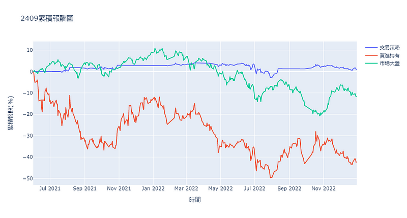
2021后半年到2022整年，对于友达来说是整体缓步向下的趋势。若采用买进持有的策略，到期日所累绩报酬为严重的-40%到-50%之间，相对的，采用布林通道交易策略之下，其表现是优于买进持有的。更甚者，虽然这一年半友达的表现不如市场大盘，然而在本次策略之下，却是优于大盘表现的。

然而单纯的布林通道策略，在下滑大趋势区段中后的回升段中，容易有过早出场的劣势，在上升区段中，容易有极少入场的窘境；故针对股价大幅变动的个股，建议多采用其他判断趋势强弱的指标，加以优化自身的策略。

温馨提醒，本次策略与标的仅供参考，不代表任何商品或投资上的建议。之后也会介绍使用TEJ资料库来建构各式指标，并回测指标绩效，所以欢迎对各种交易回测有兴趣的读者，选购TEJ E-Shop的相关方案，用高品质的资料库，建构出适合自己的交易策略。

完整程式码

点此前往Github