目录
追逐利益、趋避风险是投资人的目标,预测股价动是达成上述目标的方法之一。过去人们使用ARIMA、GARCH等时间序列,试图刻画出未来股价的轨迹。到了今日,随著深度学习的蓬勃发展,越来越多时间序列相关的模型的出现,似乎能应用于未来股价的预测中。本文即是利用GRU与LSTM两序列相关模型进行股价预测,使用前5日的开盘、最高、最低、收盘价预测隔日收盘价。
过去【资料科学】LSTM已对LSTM有相当程度的介绍,于此不在多做赘述。本文多加入了同样是RNN家族的GRU模型,检验GRU与LSTM在股价预测上的表现差异。GRU改动了LSTM中记忆单元的遗忘、输入与输出门,将其缩编为更新门与重置门,前者类似于LSTM中的遗忘与输入门,负责决定每次迭代需保留与丢弃的信息,后者则是决定需丢弃过去累积的信息。从三门减少至双门的情况下,GRU相较于LSTM能达成较快的运算速度,且其表现理论上不亚于LSTM。
本文使用Google Colab作为编辑器
# 载入所需套件
import pandas as pd
import numpy as np
from sklearn.preprocessing import StandardScaler
import plotly.graph_objects as go
import os
import time
import tejapi
import math
import torch
from torch import nn, optim
from torch.utils.data import Dataset, DataLoader, TensorDataset

# 登入TEJ API
api_key = 'YOUR_KEY'
tejapi.ApiConfig.api_key = api_key
tejapi.ApiConfig.ignoretz = True

# 载入gpu
device = torch.device('cuda' if torch.cuda.is_available() else 'cpu')
公司交易面资料库: 未调整股价(日),资料代码为(TWN/APRCD)。
使用台积电(2330.tw)未调整开盘、最高、最低与收盘价格,时间区间为2019/01/01到2023/01/01。先进行标准化,再将其依照8:2进行训练与验证集切分。标准化能有效减少特征规模大小不均所造成的偏误且能加速训练时间。
# 股价
gte, lte = '2019-01-01', '2023-01-01'
data = tejapi.get('TWN/APRCD',
                   paginate = True,
                   coid = '2330',
                   mdate = {'gte':gte, 'lte':lte},
                   opts = {
                       'columns':[ 'mdate', 'open_d', 'high_d', 'low_d', 'close_d', 'volume']
                   }
                  )
# 标准化
scaler = StandardScaler()
data = scaler.fit_transform(data)

# 训练与验证集
train, test = data[:int(0.8 * len(data)), :4], data[int(0.8 * len(data)):, :4]
建立Pytorch Dataset与DataLoader,可以自动建置Batch以方便后续将资料喂给模型训练。
def create_dataset(dataset, lookback):
    X, y = [], []
    for i in range(len(dataset)-lookback):
        feature = dataset[i:i+lookback, :]
        target = dataset[i+1:i+lookback+1][-1][-1]
        X.append(feature)
        y.append(target)
    return torch.FloatTensor(X).to(device), torch.FloatTensor(y).view(-1, 1).to(device)

lookback = 5 # 设定前五天股价预测下一日
X_train, y_train = create_dataset(train, lookback = lookback)
X_val, y_val = create_dataset(test, lookback = lookback)
loader = DataLoader(TensorDataset(X_train, y_train), shuffle = False, batch_size = 32)
模型架构为一层LSTM,加上一层Dropout后,再接上一个全连接层。加入Dropout的原因为防止模型产生过拟合问题。
● input_size: 为输入的特征数量,使用开盘、最高、最低与收盘价格,故 input_size = 4。
● hidden_size: 为LSTM隐藏层神经元数。
● num_layer: LSTM层数,单层预设为一。
● batch_first: 输出维度保持(batch_size, sequence_len, hidden_size),其中 sequence_len为5,因为我们采用五天价格预测隔日价格。
# 建立单层LSTM函式
class S_LSTM(nn.Module):
    def __init__(self):
        super().__init__()
        self.lstm1 = nn.LSTM(input_size = 4, hidden_size=64, num_layers=1, batch_first=True)
        self.dropout = nn.Dropout(0.2)
        self.linear = nn.Linear(64, 1)
    def forward(self, x):
        x, _ = self.lstm1(x)
        x = self.dropout(x)
        x = x[:, -1, :]
        x = self.linear(x)
        return x

# 建立训练流程函式
def trainer(epochs, loader, X_train, y_train, X_val, y_val, model, criterion, optimizer):
  train_loss, test_loss = [],[]
  for epoch in range(epochs):
    model.train()
    for batch, (x, y_true) in enumerate(loader):
      y_pred = model(x)
      loss = criterion(y_pred, y_true)
      loss.backward()
      optimizer.step()
      optimizer.zero_grad()
    model.eval()
    with torch.no_grad():
      y_pred = model(X_train)
      train_rmse = np.sqrt(criterion(y_pred, y_train).item())
      train_loss.append(train_rmse)
      y_pred = model(X_val)
      test_rmse = np.sqrt(criterion(y_pred, y_val).item())
      test_loss.append(test_rmse)
      if (epoch+1) % 100 == 0:
        print('epoch %d train rmse %.4f test rmse %.4f' % (epoch+1, train_rmse, test_rmse))
  return train_loss, test_loss

# 设置模型、损失函数与优化器
model = S_LSTM().to(device)
criterion = nn.MSELoss()
optimizer = optim.Adam(model.parameters())
epochs = 1000

# 开始训练并且计算训练所需时间
start = time.time()
slstm_train_loss, slstm_test_loss = trainer(epochs, loader, X_train, y_train, X_val, y_val, model, criterion, optimizer)
end = time.time()
print('single lstm time cost %.4f' %(end-start))
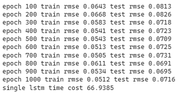
fig = go.Figure()
fig.add_trace(go.Scatter(x=np.arange(epochs), y=slstm_train_loss,
                    mode='lines',
                    name='Train Loss'))
fig.add_trace(go.Scatter(x=np.arange(epochs) , y=slstm_test_loss,
                    mode='lines',
                    name='Validation Loss'))
fig.update_layout(
    title="Loss curve for single lstm",
    xaxis_title="epochs",
    yaxis_title="rmse"
)
fig.show()
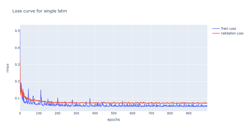
从损失曲线图可以发现约莫在第200次epoch时,验证集的损失已经趋于收敛且坐落于约莫0.07的位置,后续再将股价预测图绘制检验模型的预测能力。
train_plot = np.ones_like(data[:, 3]) * np.nan
test_plot = np.ones_like(data[:, 3]) * np.nan
with torch.no_grad():
  # 预测训练集资料
  y_pred = model(X_train)
  train_plot[lookback:int(0.8 * len(data))] = y_pred.view(-1).cpu()
  # 预测验证集资料
  y_pred = model(X_val)
  test_plot[int(0.8 * len(data))+lookback:] = y_pred.view(-1).cpu()

fig = go.Figure()
fig.add_trace(go.Scatter(x=mdate, y=train_plot,
                    mode='lines',
                    name='Train'))
fig.add_trace(go.Scatter(x=mdate , y=test_plot,
                    mode='lines',
                    name='Validation'))
fig.add_trace(go.Scatter(x=mdate , y=data[:, 3],
                    mode='lines',
                    name='True'))
fig.update_layout(
    title="Stock prediction for sngle lstm",
    xaxis_title="dates",
    yaxis_title="standardised stock"
)
fig.show()
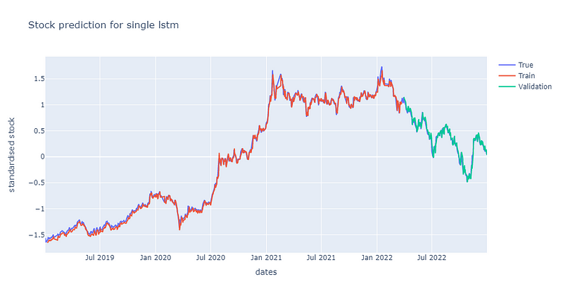
从上图与损失曲线图可以发现单层LSTM对于股价的预测能力是相当不错的。这点十分有趣,因为根据【资料科学】LSTM所述,他们在单层的LSTM表现是较差的,并无法完整捕捉到时间序列资讯。而我们与他们的区别在于他们有多采用每日成交量作为输入资料的特征、我们的LSTM层输出维度是64而他们的是32,Dropout的比率我们是20%而他们的是30%。目前认为最有可能造成差异的原因应该为他们多采用了每日成交量作为输入特征。
虽然单层LSTM已经可以达成不错的效果,但我们不彷多堆叠几层LSTM去试看看是否能继续最佳化。多层LSTM的架构为: 一层LSTM + 一层Dropout + 一层LSTM + 一层Dropout + 一层全连接层。其中两次Dropout的比率都调整为40%,这里将比率调高的原因是为了避免过拟合问题。
# 建立双层LSTM函式
class LSTM(nn.Module):
    def __init__(self):
        super().__init__()
        self.lstm1 = nn.LSTM(input_size = 4, hidden_size=64, num_layers=1, batch_first=True)
        self.dropout1 = nn.Dropout(0.4)
        self.lstm2 = nn.LSTM(input_size = 64, hidden_size=32, num_layers=1, batch_first=True)
        self.dropout2 = nn.Dropout(0.4)
        self.linear = nn.Linear(32, 1)
    def forward(self, x):
        x, _ = self.lstm1(x)
        x = self.dropout1(x)
        x, _ = self.lstm2(x)
        x = self.dropout2(x)
        x = x[:, -1, :]
        x = self.linear(x)
        return x
# 建立训练流程函式
def trainer(epochs, loader, X_train, y_train, X_val, y_val, model, criterion, optimizer):
  train_loss, test_loss = [],[]
  for epoch in range(epochs):
    model.train()
    for batch, (x, y_true) in enumerate(loader):
      y_pred = model(x)
      loss = criterion(y_pred, y_true)
      loss.backward()
      optimizer.step()
      optimizer.zero_grad()
    model.eval()
    with torch.no_grad():
      y_pred = model(X_train)
      train_rmse = np.sqrt(criterion(y_pred, y_train).item())
      train_loss.append(train_rmse)
      y_pred = model(X_val)
      test_rmse = np.sqrt(criterion(y_pred, y_val).item())
      test_loss.append(test_rmse)
      if (epoch+1) % 100 == 0:
        print('epoch %d train rmse %.4f test rmse %.4f' % (epoch+1, train_rmse, test_rmse))
  return train_loss, test_loss
# 设置模型、损失函数与优化器
model = LSTM().to(device)
criterion = nn.MSELoss()
optimizer = optim.Adam(model.parameters())
epochs = 1000
# 开始训练并且计算训练所需时间
start = time.time()
lstm_train_loss, lstm_test_loss = trainer(epochs, loader, X_train, y_train, X_val, y_val, model, criterion, optimizer)
end = time.time()
print('stack lstm time cost %.4f' %(end-start))
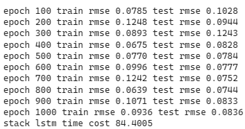
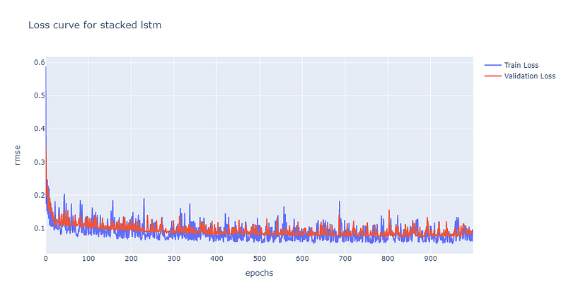
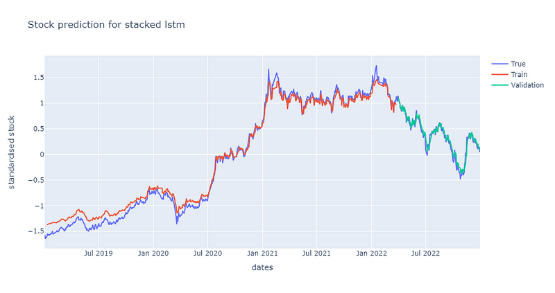
可以发现随著模型复杂度提高,收敛的速度下滑到约500个epoch才有收敛到0.1的迹象,且随后的震荡也相较於单层LSTM为大。后续再将股价预测图绘制检验模型的预测能力,可以发现预测能较不如单层LSTM,但也能抓出涨跌趋势,绘图程式码请见最下方。
接著我们使用GRU模型预测股价,一样先加上一层GRU层,在叠上一层比率为0.2的Dropout跟全连接层。
# 建立单层GRU函式
class S_GRU(nn.Module):
def __init__(self):
super().__init__()
self.gru1 = nn.GRU(input_size = 4, hidden_size=64, num_layers=1, batch_first = True)
self.dropout = nn.Dropout(0.2)
self.linear = nn.Linear(64, 1)
def forward(self, x):
x, _ = self.gru1(x)
x = self.dropout(x)
x = x[:, -1, :]
x = self.linear(x)
return x
# 建立训练流程函式
def trainer(epochs, loader, X_train, y_train, X_val, y_val, model, criterion, optimizer):
train_loss, test_loss = [],[]
for epoch in range(epochs):
model.train()
for batch, (x, y_true) in enumerate(loader):
y_pred = model(x)
loss = criterion(y_pred, y_true)
loss.backward()
optimizer.step()
optimizer.zero_grad()
model.eval()
with torch.no_grad():
y_pred = model(X_train)
train_rmse = np.sqrt(criterion(y_pred, y_train).item())
train_loss.append(train_rmse)
y_pred = model(X_val)
test_rmse = np.sqrt(criterion(y_pred, y_val).item())
test_loss.append(test_rmse)
if (epoch+1) % 100 == 0:
print('epoch %d train rmse %.4f test rmse %.4f' % (epoch+1, train_rmse, test_rmse))
return train_loss, test_loss
# 设置模型、损失函数与优化器
model = S_GRU().to(device)
criterion = nn.MSELoss()
optimizer = optim.Adam(model.parameters())
epochs = 1000
# 开始训练并且计算训练所需时间
start = time.time()
sgru_train_loss, sgru_test_loss = trainer(epochs, loader, X_train, y_train, X_val, y_val, model, criterion, optimizer)
end = time.time()
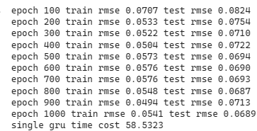
print('single gru time cost %.4f' %(end-start))
绘制损失曲线
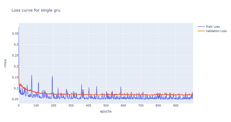
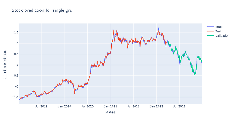
同样在epoch为200左右时,单层GRU模型的损失收敛到约0.7的位置,然而值得注意的是,其训练损失的震荡幅度较大。后续再将股价预测图绘制检验模型的预测能力,同样可发现其预测能力也是较佳的,绘图程式码请见最下方。
如同LSTM, 我们也堆叠了一个双层GRU模型检验是否能达成更佳的预测效果。模型架构: 一层GRU + 一层Dropout + 一层GRU+ 一层Dropout + 一层全连接层。其中两次Dropout的比率都调整为40%,这里将比率调高的原因是为了避免过拟合问题。
# 建立双层GRU函式
class GRU(nn.Module):
    def __init__(self):
        super().__init__()
        self.gru1 = nn.GRU(input_size = 4, hidden_size=64, num_layers=1, batch_first=True)
        self.dropout1 = nn.Dropout(0.4)
        self.gru2 = nn.GRU(input_size = 64, hidden_size=32, num_layers=1, batch_first=True)
        self.dropout2 = nn.Dropout(0.4)
        self.linear = nn.Linear(32, 1)
    def forward(self, x):
        x, _ = self.gru1(x)
        x = self.dropout1(x)
        x, _ = self.gru2(x)
        x = self.dropout2(x)
        x = x[:, -1, :]
        x = self.linear(x)
        return x
# 建立训练流程函式
def trainer(epochs, loader, X_train, y_train, X_val, y_val, model, criterion, optimizer):
  train_loss, test_loss = [],[]
  for epoch in range(epochs):
    model.train()
    for batch, (x, y_true) in enumerate(loader):
      y_pred = model(x)
      loss = criterion(y_pred, y_true)
      loss.backward()
      optimizer.step()
      optimizer.zero_grad()
    model.eval()
    with torch.no_grad():
      y_pred = model(X_train)
      train_rmse = np.sqrt(criterion(y_pred, y_train).item())
      train_loss.append(train_rmse)
      y_pred = model(X_val)
      test_rmse = np.sqrt(criterion(y_pred, y_val).item())
      test_loss.append(test_rmse)
      if (epoch+1) % 100 == 0:
        print('epoch %d train rmse %.4f test rmse %.4f' % (epoch+1, train_rmse, test_rmse))
  return train_loss, test_loss
# 设置模型、损失函数与优化器
model = GRU().to(device)
criterion = nn.MSELoss()
optimizer = optim.Adam(model.parameters())
epochs = 1000
# 开始训练并且计算训练所需时间
start = time.time()
gru_train_loss, gru_test_loss = trainer(epochs, loader, X_train, y_train, X_val, y_val, model, criterion, optimizer)
end = time.time()
print('stack gru time cost %.4f' %(end-start))
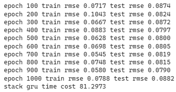
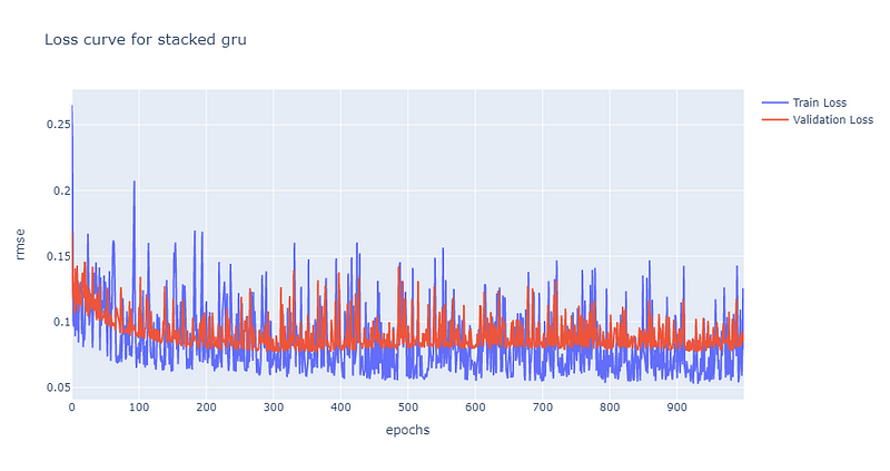
可发现双层GRU的震荡幅度较单层大,约莫在300个epoch渐渐收敛到约0.7的位置。后续再将股价预测图绘制检验模型的预测能力,同样可发现其预测能力较单层逊色,绘图程式码请见最下方。
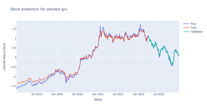
从上述结果可以发现,不论是LSTM或是GRU,单层在台积电股价预测上表现皆优于双层。接著我们比较两单层模型在验证集的损失曲线,可以发现两者最后都能收敛到0.07附近。在震荡部分事实上两者幅度相当,但GRU在前期的损失下降幅度明显大于LSTM,绘图程式码见最下方。
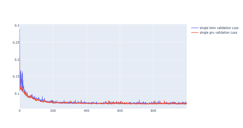
此外,GRU理论上来说,运算速度会快于LSTM,而在训练过程中,也发现这样的事实,单层GRU相较於单层LSTM快约8秒,双层GRU则快双层LSTM约3秒,见下方萤光色域。
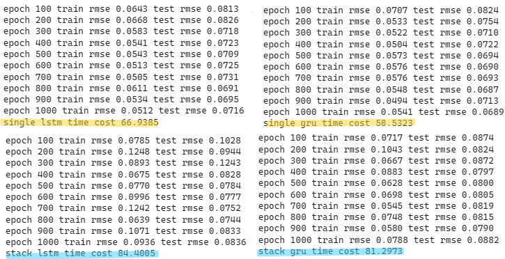
总的说,LSTM与GRU在这次的试验中,对台积电股价皆有一定的预测能力,然而GRU受惠于演算法结构优化,在计算上所需时间较短。由于这次试验仅采取单一股票标的且时间限缩于2019到2022三年,故无法说明LSTM或GRU对于股价一定具有预测能力。但根据【资料科学】LSTM的结论与本次的观察,我们认为LSTM与GRU可以作为投资人在选股时的一项参考依据,建议可以搭配其他选股指标,比如: 【实战应用】布林通道交易策略 或 【量化分析】MACD指标回测实战,建构投资策略。
温馨提醒,本次策略与标的仅供参考,不代表任何商品或投资上的建议。之后也会介绍使用TEJ资料库来建构各式指标,并回测指标绩效,所以欢迎对各种交易回测有兴趣的读者,选购TEJ E-Shop的相关方案,用高品质的资料库,建构出适合自己的交易策略。